Contents
Add
dataset to the Dataset list
Initialise
app
The first time you open the app (.exe in in DichroIDP/DichroIDP folder) there will no datasets in the dataset list box.
1. Click on the + sign next to the list box.
2. On the dialog click 'browse'.
3. Navigate to the dataset folder (in the first DichroIDP folder).
4. Open the dataset folder and select IDP175, BUT DONT OPEN IT.
5. Click on 'select folder’ then click ‘Ok’.
It will now be in the list. Repeat the procedure to add the SP175
dataset to the list. Whichever dataset is showing in the list box is used for
the calculation
you only do this the first time you open the app unless you move it to another location
on your computer.
File types
1) DichroApp can read .gen files generated by CDtoolX and CDTool and two column text files where column x is the wavelength and column y holds CD data. The columns should be tab-delimited.
2) A spectrum should have a high wavelength of 240nm or above or it will not be accepted.
3) A spectrum should have a wavelength interval of 1 or 0.5 nm or it will not be accepted.
4) If the interval is 0.5 nm the high wavelength must be a whole number of it will not be accepted.
5) The lowest wavelength analysed is determined by the low wavelength of the dataset, the lowest wavelength of the query data or the lowest wavelength chosen by the user. For a good analysis 190 nm or below is recommended.
Analysing
a spectrum
1) Choose the file type by clicking the appropriate radio button next to the ‘Open spectrum’ button.
2) Click the open spectrum button and navigate to the spectrum file
3) Select a dataset from the Dataset list
4) Select the low wavelength cut-off of your spectrum. If this is below the low wavelength of the dataset or above it, either the query data or the dataset data will be automatically truncated. If the value is below that of your query data, the lowest wavelength of the query data is chosen by default.
6) Select the spectrum in the file list
7) Click analyse.
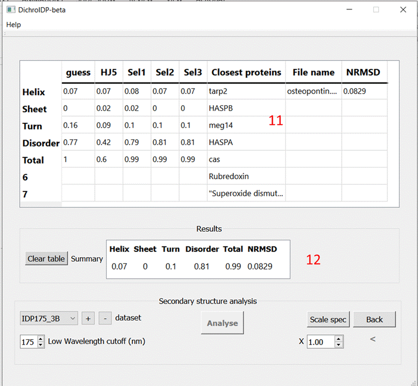
8) The results are presented in two tables which can be copied into a spread sheet by, selecting the required cells, right click and choose copy. The summary table also can be copied as above or pressing CTRL+C
9) The top table displays the results of each stage of the analysis. (Details found here)
a. The initial guess
b. HJ5 solution
f. Nine closest proteins based on RMSD (the closest is coloured green).
g. NMRSD.
10) If you get a message to say that there is no selcon3 solution the app will supply a selcon2 solution, increasing the low wavelength cutoff or scaling the spectrum is recommended.
11) A zero NRMSD indicates a failure to find a useful solution. The NRMSD will be coloured red. Increasing the low wavelength cutoff or scaling is recomended.
12) Return to the analysis page by pressing the ‘back button. If there is a Selcon3 solution, a back calculated ‘refit’ spectrum is displayed in the plot window
Scale
spectrum
1) Select the spectrum in the file list
2) Enter a scale factor in the scale entry box
3) Click scale button
4) The scaled spectrum will appear in the plot window and its file is automatically selected in the file list.
5) Click analyse.
Clear
Data
1) Analysis page
a. Selected rows (and cognate plots) can be removed by right clicking the list table and choosing ‘delete row’.
b. All plots can be cleared by choosing ‘delete all’.
2) Results page
a. Results can be cleared from both tables by clicking the ‘Cleat table’ button
Add dataset to the Dataset list
1) Custom datasets can be added to the dataset list for use by clicking the + button, select brows in the dialog box and select the new dataset folder (without opening it). Then click OK
2) The new dataset will be available in the dataset list box
3) A dataset in the list box can be removed by clicking the – button
4) To create a custom dataset copy the IDP175 dataset folder to the datasets folder and rename it. Then change the data in the four files inside
a. A.txt contains the spectral data in columns
b. F.txt contains the secondary structure assignments in columns
c. lbl1 contains the Assignment labels
d. lbl2 contains the protein names

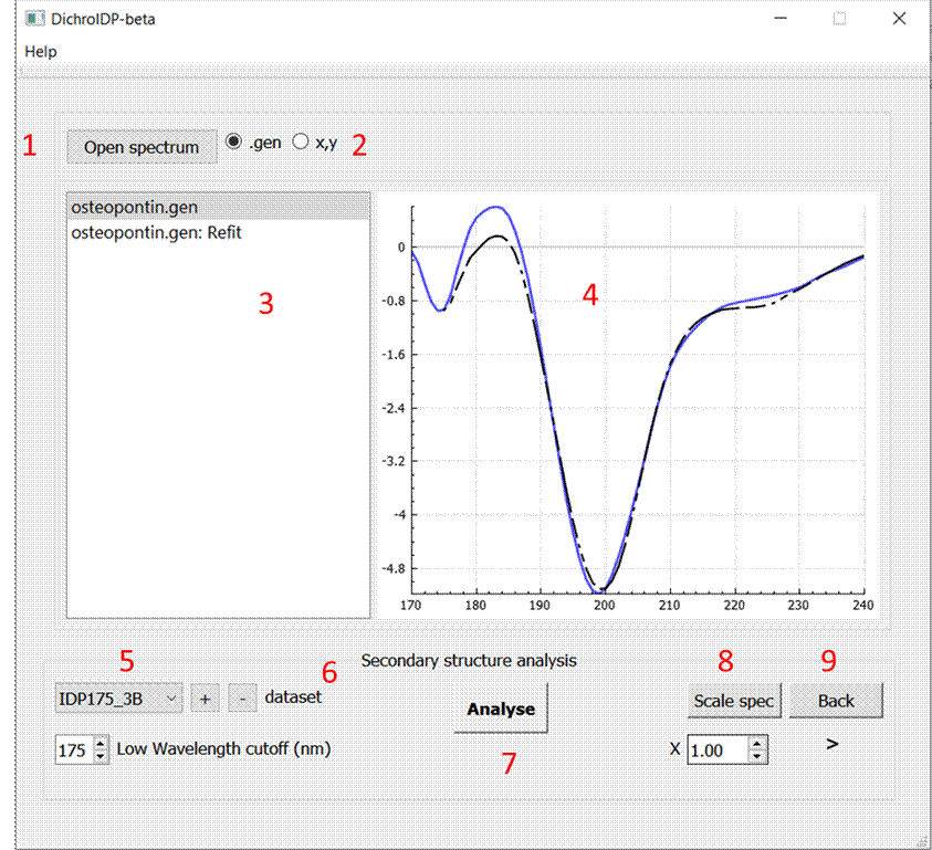
1) Open spectrum button
2) File type selection
3) File list window
4) Plot window
5) Dataset list
6) Add or remove dataset from list using + or – buttons
7) Low wavelength cutoff
8) Analysis button
9) Scale selected spectrum
10) Back button to navigate to and from results page

DichroAPP Results page
11) Full 11 Results window
12) Results summary
The Algorithm
SelD is based on Selcon3 algorithm (Sreerema & Woody1993, 1999)
We have two matrices in the dataset:
A is an m x n matrix of protein CD spectra where each column contains spectral data with m wavelengths
F is a k x n structural matrix where each column represents a protein with k structural assignments.
We need to relate structure and spectral data through the linear equation
(1) F = X A
And solve for X
Initial guess
1. First an initial guess is made:
a. The RMSD’s between the query spectrum and each spectrum in the A matrix are calculated and the A matrix columns sorted in ascending order of RMSD value.
b. The F matrix columns are then sorted to be consistent with the A matrix
c. The first column of structural assignments in the sorted F matrix represents the initial guess.
2. The query spectrum is added to the A matrix as the first column (a0), and the initial guess copied and added to the beginning of the F matrix (f0). We now have matrices Acat and Fcat (cat for catenated).
Selcon1
The linear equation to solve is now (2) Fcat=X Acat
3.
a. SVD
is performed on Acat
to give (3) Acat
= U S VT
b. Substituting
3 into 2 and solving for X gives (4) X=
Fcat V S+ Ut
where S+ is the
inverse of S
4.
a. The diagonal entries of S are the singular values, and, since only a few singular values are required to reconstruct the spectrum within experimental error, only the first 7 values are considered (Ns).
b. Similarly, not all protein spectra contribute significantly.
c. So a number of solutions to X are generated by repeating equations 3 and 4 using 3 to Np+1 proteins and Ns =1 to Np-2 or 7, whichever is smaller (Where Np is the number of spectra used).
5. The sum-frac rule is then used: Only solutions which satisfy |∑fk -1|<=0.5 and fk >=-0.025 are considered (i.e the sum of the structural fractions in retained solutions are constrained to be close to 1).
6. Then for each value of Np the solution with fk closest to 1 is retained.
7. These solutions are averaged and replace f0, the first column of Fcat (the approximation).
8. The process is reiterated using further approximations (f0) until the RMSD between successive solutions is < 0.0025
9. The final solution is the selcon1 solution
Selcon2
10. All solutions from part 6 are processed as follows
a. For each singular value Sn, and protein number Np, the appropriate columns in Acat (Acat2) are deconstructed by SVD Acat2 = U S VT
b. For each Sn, a refit matrix is then reconstructed: refit= U S VT
c. The RMSD between the query spectrum and each column of the refit matrix is recorded
d. All solutions with an RMSD <=0.25 are retained and averaged to form the Selcon2 solution
Selcon3
11. Solutions in part d are subject to the helix laws before averaging to produce the selcon3 solution
12. The helix laws compare helix fractions from the HJ5 solution to selcon2 solutions.
a. Equations 3 and 4 are performed using matrix A
b. A solution for X is generated using 5 basis spectra. This is the HJ5 solution
c. The helix fraction for this solution is compared to helix fractions in the selcon2 solutions and various tests performed.
d. Those that pass the tests are averaged to form the selcon3 solution
Refitted spectrum and NMRSD
13. The refitted spectrum is generated by applying 10 above to the selcon3 solutions in 12c. Then averaging the spectra generated.
14. NMRSD between the refitted spectrum and the query is

Where CDq is the Query CD data,
and CDr is the refit CD data and n is the number
of data points.
Datasets
IDP175
To be sorted
References
Sreerema, N. and Woody, R.W. (1993) A self-consistent method for the
analysis of protein secondary structure from circular dichroism. Anal. Biochem. 209, 32-44.
Sreerema, N., Venyaminov, S.Y., and Woody,
R.W. (1999) Estimation of the number of helical and strand segments in proteins
using CD spectroscopy. Protein Sci. 8, 370-380.
Please Cite the following if you use any aspect of this programme for processing or analysing your data:
Coming soon
Contact Us
N.B. Please note that we cannot provide advise about installation on individual computers/systems.